

Personalization
Personalization is the “holy grail” of e-commerce.
Data shows that the sooner a shopper finds what they’re looking for, the more likely it is the shopper will buy it. Personalization of content feeds and search results achieves that. So brands seek to show each shopper exactly the things that interest them, interspersed with a few new items they might want, but don’t know about yet.
Because TapSpot extends across a wide span of apps and sites, KLOA is well positioned to offer personalization capability to brands alongside TapSpot search.
The model described below is a personalization utility that accompanies TapSpot search. TapSpot itself uses the utility to re-rank word predictions and query suggestions according to individual user profiles. KLOA’s personalization utility is available to brands to personalize their search results, as well.
The utility emulates two models published by Pinterest: PinSage and PinnerFormer (links below).
Model part 1 — item embeddings
Emulated from PinSage paper by Rex Ying, et al: https://arxiv.org/pdf/1806.01973
The first stage determines useful representations of items. These representations are valuable for doing item-item recommendation, but also for other down-stream recommender tasks (which we will use them for).
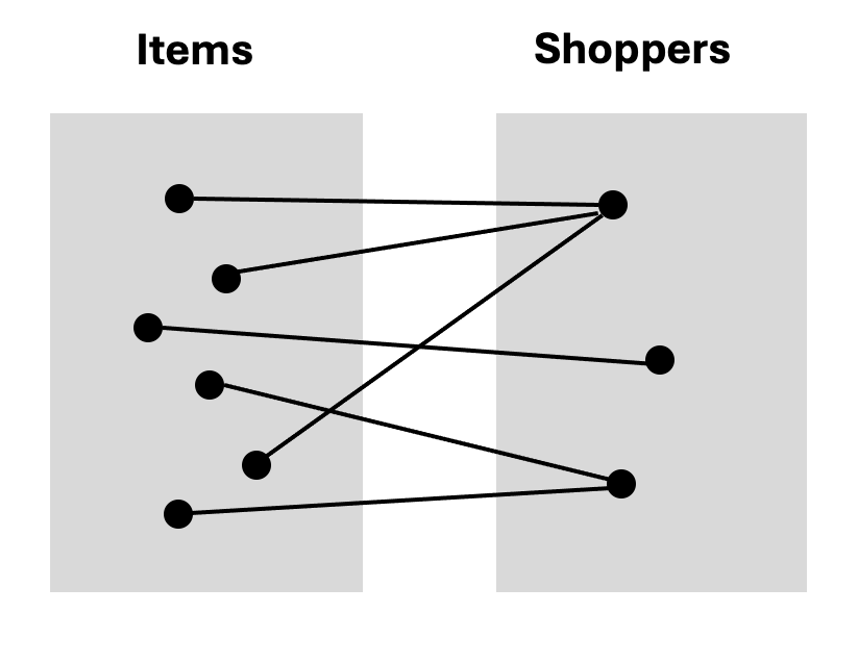
Shoppers’ interactions with items are modelled as a bipartite graph. The graph has two disjoint sets: ‘I’ contains items and ‘S’ contains shoppers. Each item is a node within the item set. Each shopper is a node in the shopper set. Any interaction (view or purchase) between an item and a shopper is an edge between those two nodes.
In addition to the graph structure, each node is associated with real-valued attributes represented in d-dimensional space. Each dimension is a feature of the item and can be either text or an image. These attributes are the content information. The goal is to leverage both attributes and the structure of the graph to generate representative embeddings for each item and shopper.
Deep learning is an effective way to find representative embeddings for each node.
For a graph, convolutional transformation of representations of neighboring nodes can capture the latent information in the graph in lower dimensional space. Broadly speaking, building a graph convolutional network (GCN) has two stages: selection of which neighboring nodes to include in convolutions for a given target and the convolution itself.
The core of the algorithm is a localized convolution operation. The root is transformation of aggregated representations from neighboring nodes through a learned dense neural network.
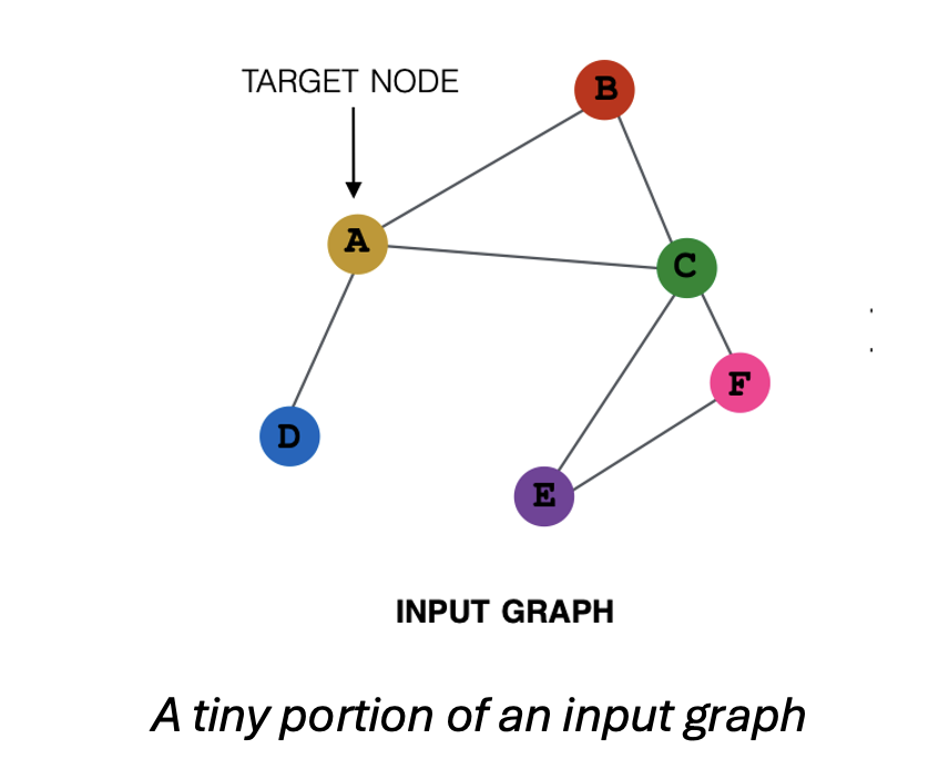
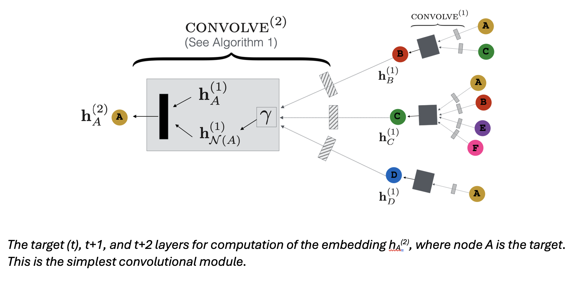
A random walk algorithm with importance pooling decides from which nodes in the neighborhood u embeddings will be taken. For each node along the random walk, an importance pooling function computes the L1-normalized visit count. The T nodes with the highest normalized visit counts have their embeddings included in the convolution.
The embedding generated for each target node benefit from both the pooling function, which incorporates edge information into the embedding, and the embeddings of each included node (content information). Together, these embed each node representation with latent info from the graph that’s useful in down-stream ranking tasks.
Training uses labeled pairs of items (q, i), where q is a query item, i is an item. The pairs are selected so that i is a good recommendation for the query item, q. The goal of training is to make the output embeddings of pairs as close as possible.
Training uses a max-margin loss function. We maximize the inner product of embeddings of positive examples, i.e., for a query item and item that are related. The inner product between a query item and an item that are unrelated should be small.
After training, the model can be used to generate embeddings for any item. The embeddings generated can be used for downstream recommendation tasks. One use (and the most direct one) is K-nearest neighbor (KNN) lookups in the learned embedding space for a given query item q.

Model part 2 — shopper embeddings from sequential data
Emulated from PinnerFormer paper by Nikil Pancha, et al: https://arxiv.org/pdf/2205.04507
Shoppers provide feedback about their interests through interaction. Examples of interactions of a shopper with items are: purchases, adds-to-basket, clicks on a product page, clicks through to an underlying link, selects of an image to zoom in on it, and others.
To personalize a shopping experience, we represent each user as a learned embedding. Because user interaction is sequential in nature (i.e., occurs over time), sequential models make sense. They aim to predict a user’s next action from all actions leading up to that point.
A solution is an end-to-end learned representation based on past interaction. The solution uses a dense all-action loss. The embedding captures a shopper’s longer-term interests, not just their likely next action. As such, the embedding can be computed offline, in a batch setting, which simplifies infrastructure.
Our solution is designed to yield a shopper representation that’s useful for a variety of downstream recommender tasks. Although an offline, batch-calculated representation is a compromise, the tradeoff is worthwhile for the reduction in complexity.
One design choice is whether to calculate for multiple embeddings or a single embedding to represent each shopper. To reduce the costs of training and inference loads, including latency, we choose to use a single embedding for all a shopper’s interests. We expect the embedding is still capable of reflecting a shopper’s varied interests. We also choose to do, offline, daily inferred updates, instead of real-time updates, to save complexity and computational cost.
Problem setup
Our interaction data is a corpus of e-commerce items I and a set of shoppers S.
For each item, we have a 256-d embedding taken as output from the model in Part I. An item representation is an aggregation of item query, shopper profile, earlier shopper-item interaction data, and associated item content (image, text).
For each shopper, we have a sequence of item interactions AS, e.g., purchases, adds-to-basket, clicks on a product page, clicks through to an underlying link, or zoom-ins. Interactions are ordered by timestamp. We take the most recent M interactions in the total history Z. With this, each action can be represented by: (a) the item embedding with which the interaction occurred, and (b) a bit of metadata that identifies the kind of interaction.
The overall aim is to learn a shopper representation f : S -> Rd compatible with the item representation g : I -> Rd, using cosine similarity to make the comparison. Said another way, we want to find representations for shoppers and items that, in vector space, optimally: (a) minimize the distance of shoppers and items that dointeract, and (b) maximize that distance for shoppers and items that do not.
In training, f and g are learned jointly, with the most recent M interaction history from AS as input. If AS has positive and negative interactions, only the positive interactions are used.
The training objective is a model that predicts positive engagement in the14 days following embedding creation, not just the next action. Stated mathematically, the objective is to learn embeddings for shopper siand item ii such that if d(sk, ii) < d(sk, ij), then ii is more likely to be of interest than ij to a shopper represented by sk over the 14 days after sk is generated.
Feature encoding
For each action in a shopper’s sequence, we have two pieces of info: item representation from Part I and metadata characterizing the interaction, e.g., kind of action, device/context for where action occurred, timestamp, and duration.
Metadata of the interaction is encoded as follows. For:
(a) kind of action, and
(b) device/context for where action occurred, we create a small, separate learnable embedding
(c) duration, we use a scalar, log (duration)
(d) timestamp, we create two derived values
(i) elapsed time since last interaction, and
(ii) time gap between actions
For (d), we use sine and cosine transformations similar to Time2vec, but with P fixed periods, rather than learned periods, and a log transformation of time, rather than linear.
The features resulting from (a), (b), (c) and (d) are concatenated to make a single vector of dimension Din. Each action Ai is denoted as ai from among RDin.
Model architecture
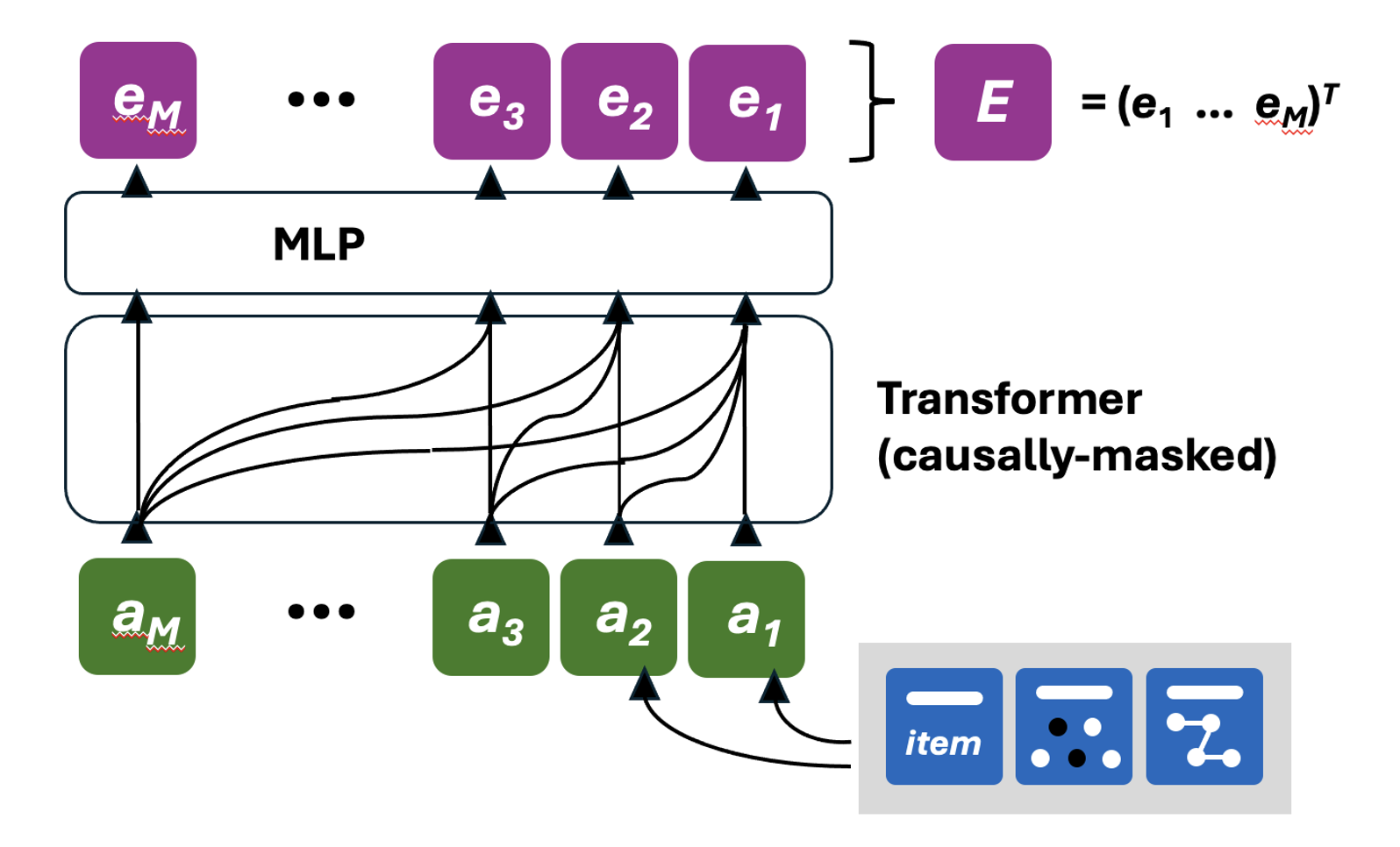
We use a transformer architecture to model the sequence of actions, using PreNorm residual connections and applying Layer Normalization before each block.
We construct the input matrix A = (a(T) … a(T-M+1))^T from among RMxDin, as follows:
use the M actions leading up to action A(T+1) as the user’s sequence
project each action aT to the transformer’s hidden dimension
add a learnable positional encoding
apply a standard transformer, consisting of:
alternating feedforward network (FFN)
multi-head self attention (MHSA) blocks
output at every position is:
passed through a small MLP, then
L2 normalized
The result is a set of embeddings E = (e(1) … e(M))^T from among R^ZxD, where Z is all the actions a shopper has taken, M is the most recent actions taken, and D is the final embedding dimension. Each embedding represents an action a shopper has taken.
Also, for each action, there is an associated item I on which the action is taken. The initial representations for these are the embeddings learned in Part I. We proceed to:
feed these to the MLP network, and
L2 normalize the output
Metric learning
Training uses shopper-item pairs. Only positive engagement is recognized. There are no examples of negative engagement. Therefore, the examples are interaction (positive) and no interaction (negative).
In selecting negative examples, there are two sources: in-batch negatives and random negatives.
an in-batch negative is a shopper-item pair not seen within the batch of training data
a random negative is a shopper-item pair not seen anywhere in the training data
We identify in-batch negatives by choosing all positive examples within the batch as negatives, then masking items that have positive engagement for that shopper. We identify random negatives by uniform sampling items from the entire corpus, again, including only those that the shopper has not interacted with. From the negative examples, we compute a set of negative embeddings. These are items not selected by the given shopper.
With these, we now have a collection a shopper embeddings s and item embeddings i. These are paired, some being positive examples and some negative, as decided by the selection process in the previous section.
The loss function is a sampled softmax with logQ correction. The correction is applied to each logit based on the probability that a given negative appears in the batch. We also learn a temperature to constrain the lower boundary for stability.

Training objective
For the loss function chosen, we now decide how to select training pairs (si, ii) to use. There are multiple forms of positive engagement, e.g., purchases, adds-to-basket, clicks on a product page, clicks through to an underlying link, or zoom-ins. In training, these are not distinguished. Any of these actions is simply considered “positive”.
Three training objectives are considered: next-action prediction, all-action prediction, dense all-action prediction. We choose dense all-action.
For dense all-action prediction, we take inspiration from SASRec and modify the all‑action objective. For this objective, rather than predicting actions over K days using only e1, we instead select a set of random indices {zi}. For each ezi, we aim to predict a randomly selected positive action from the set of all positive actions over the next K days. To avoid losing the effect of ordering, we apply causal masking to the transformer’s self‑attention block: each action may attend to only past or present actions, not future ones. To decrease memory usage, for each ezi, we aim to predict just one positive action, not all that are possible.

Model serving
With inference as an offline, batch activity, we infer the model in a daily, incremental workflow according to the figure below. In the workflow, we:
create new embeddings for any shopper who interacted with an item in the past day
merge them with the previous day’s embeddings, then
upload them to a key-value feature store for online serving
Because we: (a) generate new embeddings for only those shoppers who have engaged in the last day, and (b) run inference offline, where latency is not a constraint, we are able to use larger models than would otherwise be possible. This increases the information that embeddings can capture. Retrieval can be handled by any standard retrieval utility, e.g., SageMaker or ElasticSearch.
